GSP_DEMO_GRAPH_EMBEDDING - Demonstration file for graph embeddings

Description

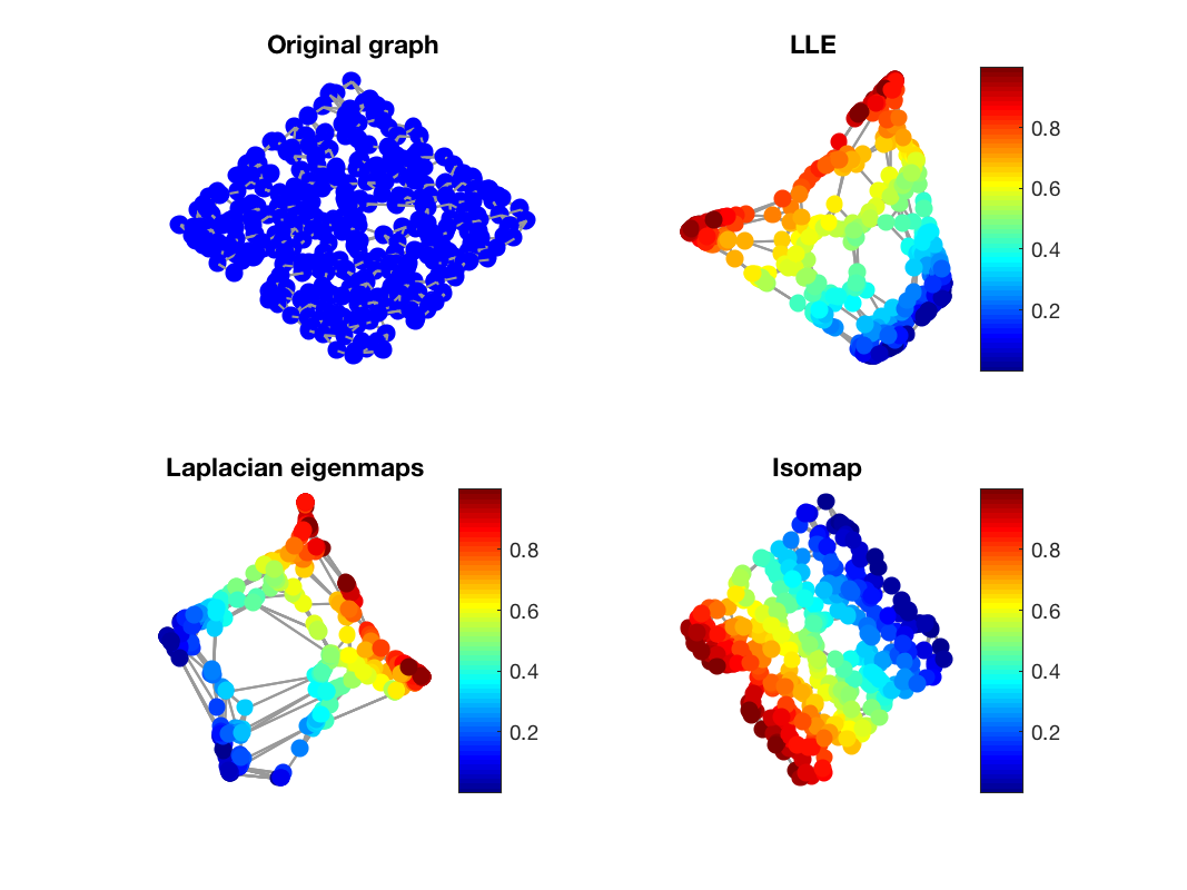
In this demo we perform a low-dimensional embedding on a specific graph using three different algorithms and we plot the resulting embeddings on a single plot. At first we create a 2-D sensor graph embedded in a 3-D space. We then compute 3 different embeddings for this graph: Laplacian eigenmaps, LLE, and Isomap.

Laplacian eigenmaps

This function uses the Laplacian of the graph and the diagonal degree matrix to compute the eigenvalues and eigenvectors of generalized eigenvector problem, \(L U = D U \Lambda\). The coordinates of the embedding are the eigenvectors that correspond to the bottom dim eigenvalues (ignoring always the zero eigenvalue).

Locally Linear Embedding (LLE)

This method first converts the weighed adjacency matrix to a distance matrix. Then it computes another weight matrix \(A\) by minimizing each reconstruction error \(\epsilon = \|x -\sum_j a_j x_j \|^2\) where the \(x_j\) are the neighboors of \(x\). To do so we first compute the following local covariance matrix:

\begin{equation*} C_{jk} = \frac{1}{2} (D_{\cdot j}+D_{i, \cdot}-D_{ij}-D_{\cdot \cdot}) \end{equation*}

where \(D_{ij}\) is the squared distance matrix,

\begin{equation*} D_{\cdot, j} = \frac{1}{n} \sum_i D_{ij}, \end{equation*}

\begin{equation*} D_{i,\cdot} = \frac{1}{n} \sum_j D_{ij}, \end{equation*}

\begin{equation*} D_{\cdot, \cdot} = \frac{1}{n^2} \sum_i \sum_j D_{ij}, \end{equation*}

and where \(D\) is the \(n\) by \(n\) squared distance matrix (\(D = d^2\)). One can observe that the local covariance matrix is simply a Multi-Dimensional Scaling (MDS) of the squared distance matrix \(D\).

We calculate the weight matrix \(A\) by solving the system of linear equations \(\sum_k C_{jk}a_k=1\) and rescale the weights so that any column of \(A\) sums up to \(1\). Finally the coordinates of the embedding are the eigenvectors of the matrix \(M = (I - A)^T(I - A)\). More precisely the coordinates of the embedding are the eigenvectors that correspond to the dim+1 bottom eigenvalues of M (we always ignore the first eigenvector since the first eigenvalue is always zero) leaving us with a dim dimensional embedding.

Isomap

This algorithm computes the embedding using the distance matrix \(d\). Firstly we compute the dijkstra distance of all possible nodes of the graph. We store these values squared in a matrix \(D\) where \(D_{ij}\) is the squared dijkstra distance from node \(i\) to node \(j\). Continuing we performe a MDS on the squared dijkstra matrix \(D\). This way we compute Matrix \(B\) as

\begin{equation*} B_{jk} = \frac{1}{2} \left(D_{\cdot j}+D_{i \cdot}-D_{ij} - D_{\cdot \cdot} \right). \end{equation*}

Finally the coordinates of the embedding are the eigenvectors that corespond to the top dim eigenvalues. Finaly one can scale the coordinates as \(X=\Gamma \Lambda ^{1/2}\) where \(\Lambda\) is the diagonal matrix of dim top eigenvalues of \(B\) and \(\Gamma\) is the matrix of the corresponding eigenvectors.

The signal on the graph is related to the coordinate information of the original graph and therefore allows us to evaluate the resulting embedding by looking at the smoothness of this signal on the graph.

Resulting embeddings

This code produces the following output:

GSPBox version 0.7.4. Copyright 2013-2015 LTS2-EPFL,
by Nathanael Perraudin, Johan Paratte, David Shuman and Vassilis Kalofolias

References:

L. K. Saul and S. T. Roweis. An introduction to locally linear embedding. unpublished. Available at: http://www. cs. toronto. edu/˜ roweis/lle/publications. html, 2000.

M. Belkin and P. Niyogi. Laplacian eigenmaps and spectral techniques for embedding and clustering. In NIPS, volume 14, pages 585--591, 2001.

J. B. Tenenbaum, V. De Silva, and J. C. Langford. A global geometric framework for nonlinear dimensionality reduction. Science, 290(5500):2319--2323, 2000.