GSP_DEMO_LEARN_GRAPH_LARGE - Tutorial for graph learning using the GSPBox
Description
This is a graph learning tutorial using GSP box. It deals with most aspects needed to know in order to use graph learning:
- standard graph learning [Kalofolias 2016]
- setting params automatically for given sparsity [Kalofolias, Perraudin 2019]
- setting zero-edges up-front [Kalofolias, Perraudin 2019]
- large scale graph learning [Kalofolias, Perraudin 2019]
Let's create some artificial coordinates data:
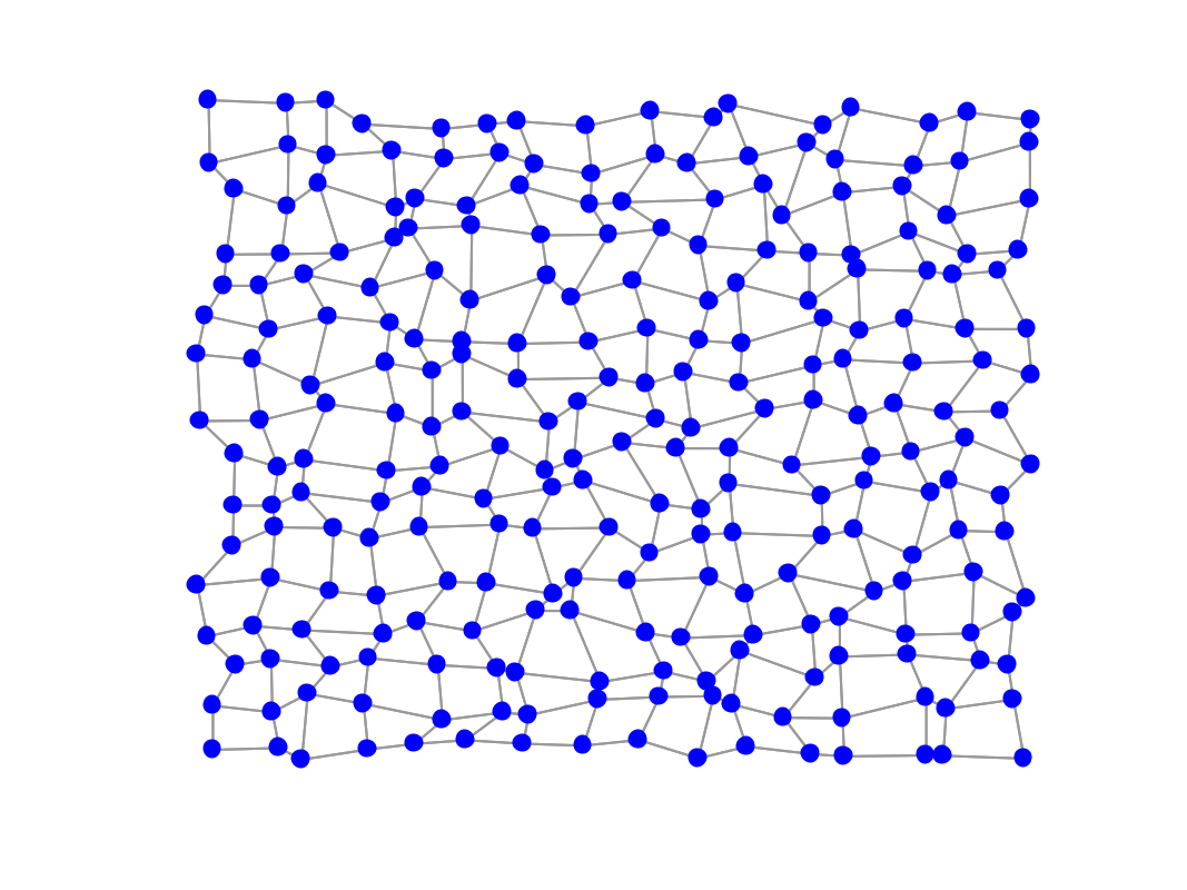
gsp_reset_seed(1);
G = gsp_2dgrid(16);
n = G.N;
W0 = G.W;
G = gsp_graph(G.W, G.coords+.05*rand(size(G.coords)));
figure; gsp_plot_graph(G);
Artificial data
Now suppose our data is the coordinates (x, y) of the points in space. Note that the data could often be a signal on these points, for example see gsp_demo_learn_graph
X = G.coords';
Right now the weights matrix W is all zeros and ones, but let's make it follow the geometry by learning weights from the new coordinates:
% First compute the matrix of all pairwise distances Z
Z = gsp_distanz(X).^2;
% this is a highly dense matrix
figure; imagesc(Z);
% Let's learn a graph, we need to know two parameters a and b according to
% [1, Kalofolias, 2016]
a = 1;
b = 1;
W = gsp_learn_graph_log_degrees(Z, a, b);
% this matrix is naturally sparse, but still has many connections unless we
% "play" with the parameters a and b to make it sparser
figure; imagesc(W);
% update weights
W(W<1e-4) = 0;
G = gsp_update_weights(G, W);
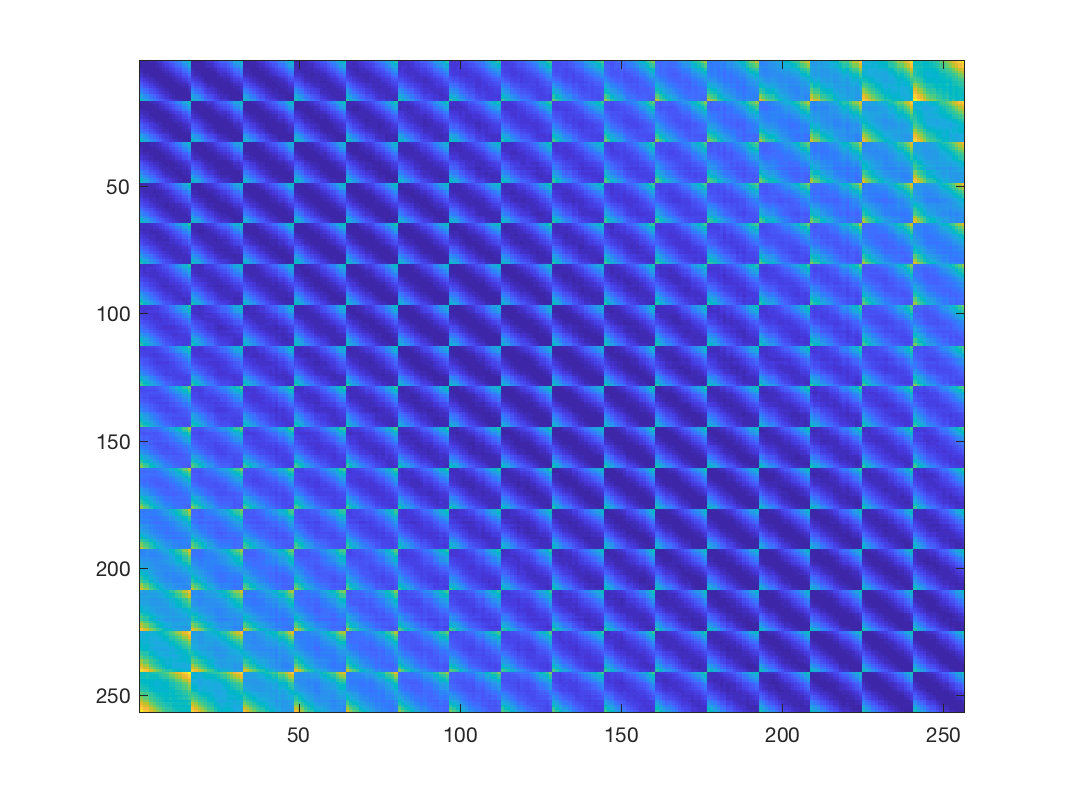
Distance matrix
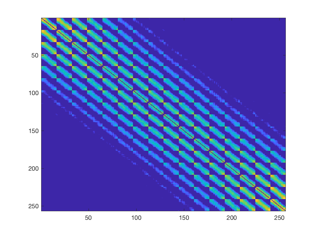
Learned weights using \(a=1\) and \(b=1\)
A practical way of setting parameters is explained in our last publication [2, Kalofolias, Perraudin 2017]. Instead of setting a and b, we need one parameter theta changing sparsity. An automatic way to find a good approximation given a desired sparsity level is with function gsp_compute_graph_learning_theta
% suppose we want 4 edges per node on average
k = 4;
theta = gsp_compute_graph_learning_theta(Z, k);
% then instead of playing with a and b, we k keep them equal to 1 and
% multiply Z by theta for graph learning:
t1 = tic;
[W, info_1] = gsp_learn_graph_log_degrees(theta * Z, 1, 1);
t1 = toc(t1);
% clean edges close to zero
W(W<1e-4) = 0;
% indeed, the new adjacency matrix has around 4 non zeros per row!
figure; imagesc(W); title(['Average edges/node: ', num2str(nnz(W)/G.N)]);
% update weights and plot
G = gsp_update_weights(G, W);
figure; gsp_plot_graph(G);
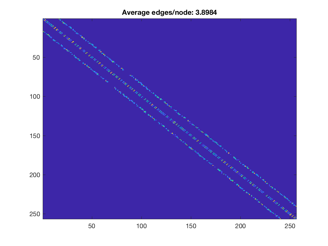
Learned weights using automatic parameter selection
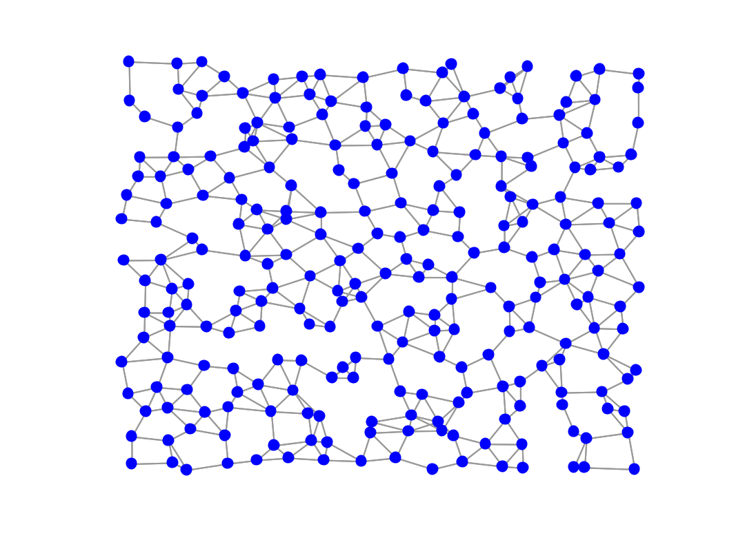
Learned graph using automatic parameter selection
An interesting feature is that we can give a pattern of allowed edges, keeping all the others to zero. This is important to add contstraints to some problems, or just to reduce computations for others:
% Suppose for example that we know beforehand that no connection could or
% should be formed before pairs of nodes with distance more than 0.02. We
% create a mask with the pattern of allowed edges and pass it to the
% learning algorithm in a parameters structure:
params.edge_mask = zero_diag(Z < 0.02);
% we also set the flag fix_zeros to 1:
params.fix_zeros = 1;
[W2, info_2] = gsp_learn_graph_log_degrees(theta * Z, 1, 1, params);
% clean edges close to zero
W2(W2<1e-4) = 0;
% indeed, the new adjacency matrix has around 4 non zeros per row!
figure; imagesc(W2); title(['Average edges/node: ', num2str(nnz(W2)/G.N)]);
% update weights and plot
G = gsp_update_weights(G, W2);
figure; gsp_plot_graph(G);
fprintf('The computation was %.1f times faster than before!\n', info_1.time / info_2.time);
fprintf('Relative difference between two solutions: %.4f\n', norm(W-W2, 'fro')/norm(W, 'fro'));
% Note that the learned graph is sparser than the mask we gave as input.
figure; subplot(1, 2, 1); spy(W2); title('W_2'); subplot(1, 2, 2), spy(params.edge_mask); title('edge mask');

Learned weights using a pattern of allowed edges

Learned graph using a pattern of allowed edges
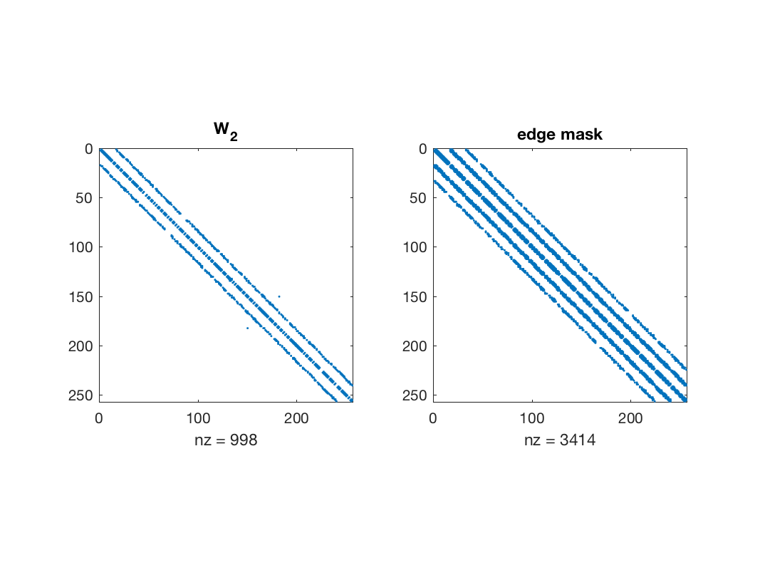
Edges selected by the algorithm
Actually this feature is the one that allows us to work with big data. Suppose the graph has n nodes. Classical graph learning [Kalofolias 2016] costs O(n^2) computations. If the mask we give has O(n) edges, then the computation drops to O(n) as well. The question is, how can we compute efficiently a mask of O(n) allowed edges for general data, even if we don't have prior knowledge? Note that computing the full matrix Z already costs O(n^2) and we want to avoid it! The solution is Approximate Nearest Neighbors (ANN) that computes an approximate sparse matrix Z with much less computations, roughly O(nlog(n)). This is the idea behind [Kalofolias, Perraudin 2017]
% We compute an approximate Nearest Neighbors graph (using the FLANN
% library through GSP-box)
params_NN.use_flann = 1;
% we ask for an approximate k-NN graph with roughly double number of edges.
% The +1 is because FLANN also counts each node as its own neighbor.
params_NN.k = 2 * k + 1;
clock_flann = tic;
[indx, indy, dist, ~, ~, ~, NN, Z_sorted] = gsp_nn_distanz(X, X, params_NN);
time_flann = toc(clock_flann);
fprintf('Time for FLANN: %.3f seconds\n', toc(clock_flann));
% gsp_nn_distanz gives distance matrix in a form ready to use with sparse:
Z_sp = sparse(indx, indy, dist.^2, n, n, params_NN.k * n * 2);
% symmetrize the distance matrix
Z_sp = gsp_symmetrize(Z_sp, 'full');
% get rid or first row that is zero (each node has 0 distance from itself)
Z_sorted = Z_sorted(:, 2:end).^2;   % first row is zero
% Note that FLANN returns Z already sorted, that further saves computation
% for computing the parameter theta.
Z_is_sorted = true;
theta = gsp_compute_graph_learning_theta(Z_sorted, k, 0, Z_is_sorted);
params.edge_mask = Z_sp > 0;
params.fix_zeros = 1;
[W3, info_3] = gsp_learn_graph_log_degrees(Z_sp * theta, 1, 1, params);
W3(W3<1e-4) = 0;
fprintf('Relative difference between two solutions: %.4f\n', norm(W-W2, 'fro')/norm(W, 'fro'));
% Note that the learned graph is sparser than the mask we gave as input.
figure; subplot(1, 2, 1); spy(W3); title('W_3'); subplot(1, 2, 2), spy(params.edge_mask); title('edge mask');
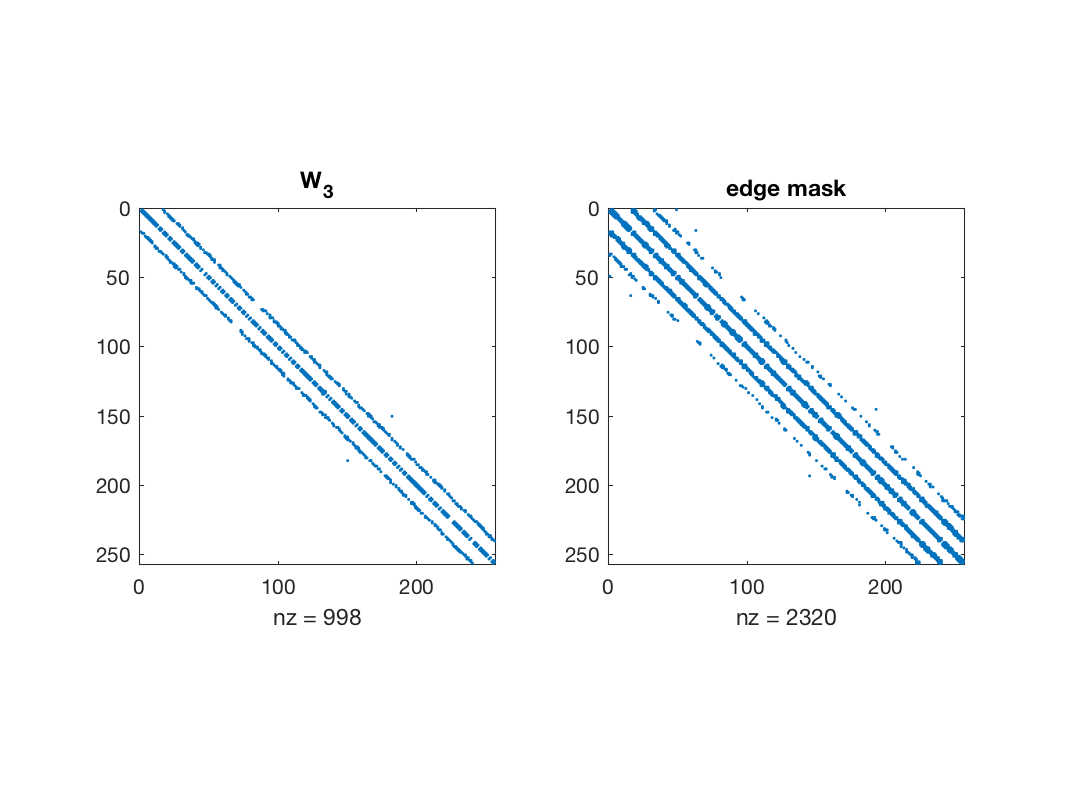
Edges selected by the algorithm
Note that we can alternatively use the vector form of Z, W, and the mask, but always AFTER symmetrizing the distance matrix Z. Make sure you use our sparse version squareform_sp.m instead of Matlab's native squareform.m, or for big graphs you might have memory issues:
z_sp = squareform_sp(Z_sp);
params.edge_mask = z_sp > 0;
% the output will be also in vectorform if the distances were in vectorform
[w3, info_3_sp] = gsp_learn_graph_log_degrees(z_sp * theta, 1, 1, params);
w3(w3<1e-4) = 0;
norm(w3 - squareform_sp(W3)) / norm(w3)
Enjoy!
This code produces the following output:
# iters:  191. Rel primal: 9.8352e-06 Rel dual: 3.5942e-08  OBJ -3.139e+02
Time needed is 0.140163 seconds
# iters:  270. Rel primal: 9.9610e-06 Rel dual: 7.6356e-06  OBJ 1.462e+02
Time needed is 0.268437 seconds
# iters:  100. Rel primal: 9.5222e-06 Rel dual: 7.8284e-06  OBJ 1.462e+02
Time needed is 0.016465 seconds
The computation was 16.3 times faster than before!
Relative difference between two solutions: 0.0003
Time for FLANN: 0.155 seconds
# iters:   88. Rel primal: 9.3082e-06 Rel dual: 7.5917e-06  OBJ 1.460e+02
Time needed is 0.012235 seconds
Relative difference between two solutions: 0.0003
# iters:   88. Rel primal: 9.3082e-06 Rel dual: 7.5917e-06  OBJ 1.460e+02
Time needed is 0.011799 seconds

ans =

     0
References:
V. Kalofolias. How to learn a graph from smooth signals. Technical report, AISTATS 2016: proceedings at Journal of Machine Learning Research (JMLR)., 2016.
V. Kalofolias and N. Perraudin. Large scale graph learning from smooth signals. International Conference on Learning Representations, 2019. [ http ]