GSP_DEMO_PYRAMID - Demonstration of the use of the graph pyramid

Description

In this demonstration file, we show how to reduce a graph using the GSPBox. Then we apply the pyramid to a simple signal.

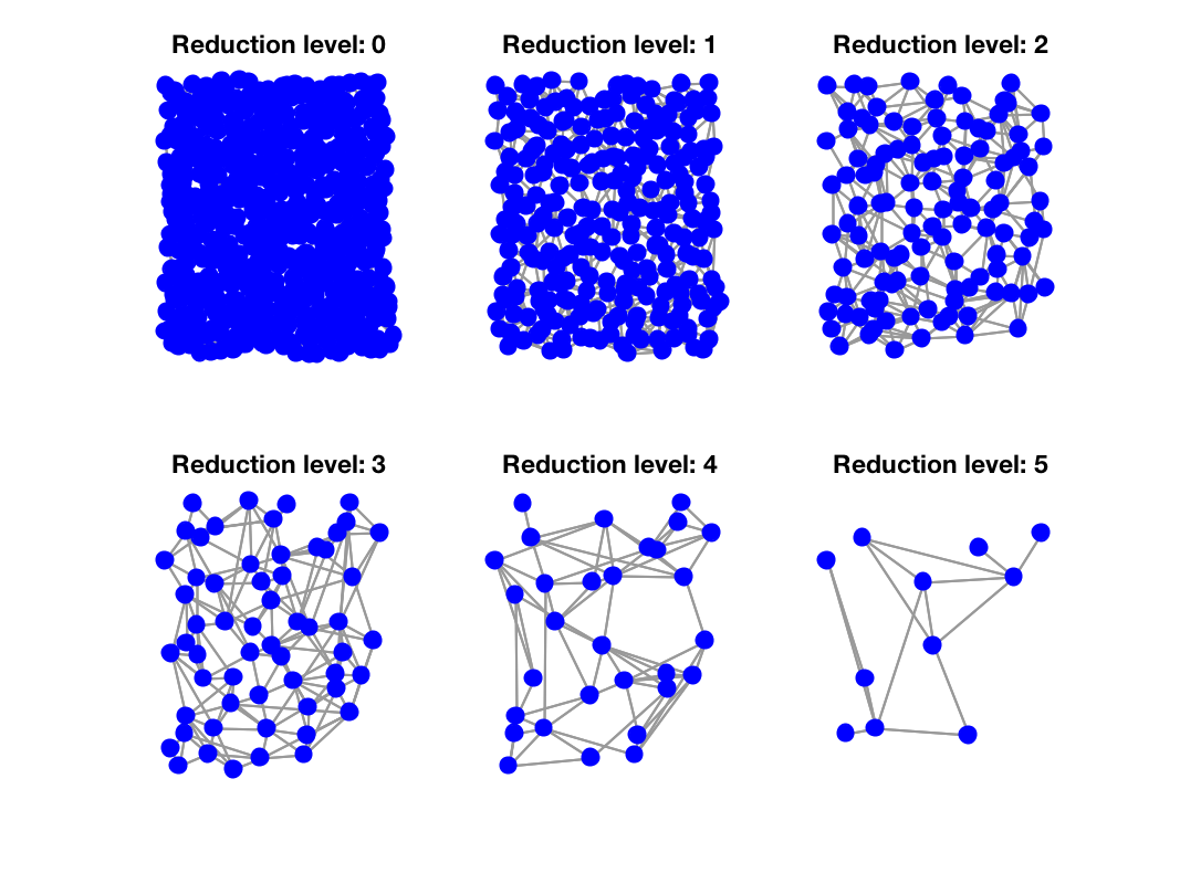
The function gsp_graph_multiresolution computes the graph pyramid for you:

param.sparsify = 1;
Gs = gsp_graph_multiresolution(G, Nlevel,param);

Gs is a cell array of graph representing the pyramid of graphs. Here all optional parameter are important:

• param.sparsify: When a graph is reduced, the density of edges has tendency to be amplified. One way to counterbalance this effect is to sparsify the graph for each sublevel. The function gsp_graph_sparsify is used to perform this operation. However, this could lead to bad graphs (disconnected for instance).
• sparsify_epsilon: Parameter epsilon used in the sparsification
• param.filters: is a cell array of filters (or a single filter). Thoses filter will be used in the analysis and synthesis operator.

Let's display the results:

figure;
for ii = 1:numel(Gs)
    subplot(2,3,ii)
    gsp_plot_graph(Gs{ii})
    title(['Reduction level: ', num2str(ii-1)]);
end

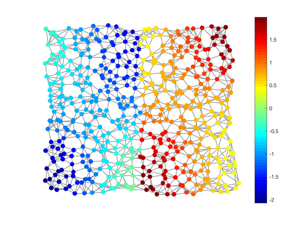
Now that we have precomputed the pyramid of graphs, we can apply it to a signal. Here we create a signal that is smooth over the graph but with a big discontinuity in the middle

The graph pyramid can be simply applied thanks to the function gsp_pyramid_analysis:

[ca,pe]=gsp_pyramid_analysis(Gs,f);

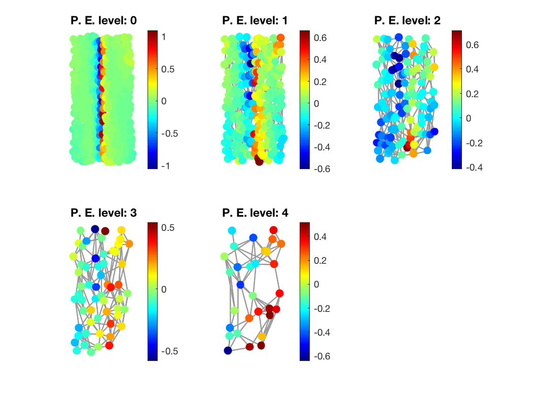
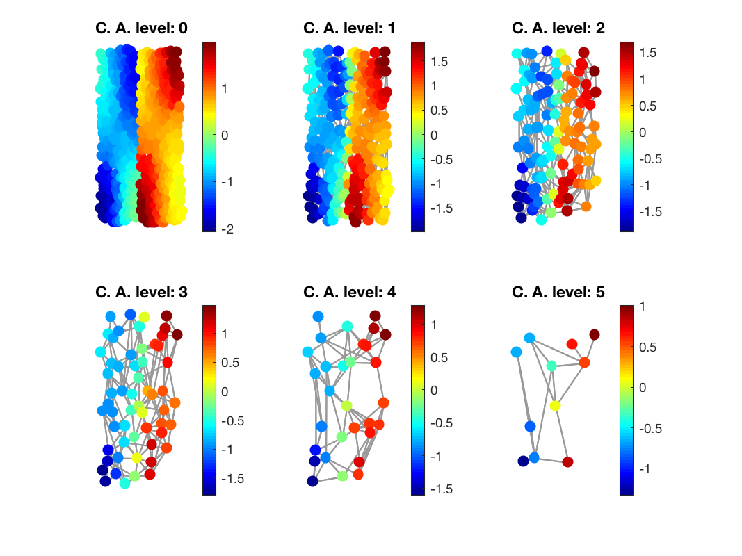
ca contains the coarse approximation of each level and pe the prediction errors. Let's display them:

figure
paramplot.show_edges = 0;
for ii = 1:numel(Gs)
    subplot(2,3,ii)
    gsp_plot_signal(Gs{ii},pe{ii},paramplot);
    title(['P. E. level: ', num2str(ii-1)]);
end

figure
for ii = 1:numel(Gs)
    subplot(2,3,ii)
    gsp_plot_signal(Gs{ii},ca{ii},paramplot)
    title(['C. A. level: ', num2str(ii-1)]);
end

Finally, you can perform a synthesis operation using the function gsp_pyramid_synthesis

coeff = gsp_pyramid_cell2coeff(ca,pe);
f_pred = gsp_pyramid_synthesis(Gs,coeff);

The function gsp_pyramid_cell2coeff remove all unecessary coefficients and keep only the last sublevel and the prediction error.

Enjoy!

This code produces the following output:

The relative reconstruction error is : 1.64455e-15