RR_TRADEOFF_SMOOTHNESS - Smoothness time frequency tradeoff
Description
Reproducible research addendum for optimization of dual gabor windows
DESIGNING GABOR DUAL WINDOWS USING CONVEX OPTIMIZATION
Paper: Nathanael Perraudin, Nicki Holighaus, Peter L. Sondergaard and Peter Balazs
Demonstration matlab file: Perraudin Nathanael
ARI -- January 2013
Dependencies
In order to use this matlab file you need the UNLocbox toolbox. You can download it on https://lts2research.epfl.ch/unlocbox and the LTFAT toolbox. You can download it on http://ltfat.sourceforge.net
The problem
It is well known that no function can be arbitrarily concentrated in both the time and the frequency domain simultaneously. When choosing a dual window to a given Gabor frame the concentration is further limited by the duality conditions, the shape and the quality of the given frame. Oversimplified, a badly conditioned Gabor frame (with large frame bound ratio \(B/A\)), admits only badly concentrated duals. However, even if the canonical dual window is well concentrated overall, applications might benefit from the improvement of time concentration versus frequency concentration and vice-versa. To see this, just recall that the TF shape of the synthesis window limits the precision of TF processing.
The following experiment demonstrates the surprising flexibility that the set of dual windows allows when choosing the appropriate TF concentration trade-off. The system parameters are the same as in Experiment 1: \(L_g = 240\), \(a = 50\), \(M=300\) and dual window support less or equal to \(L_h = 600\). However, to provide a more diverse set of examples, we exchanged the Tukey window for an Itersine window. We selected the time and frequency gradient priors to control the TF spread and optimize
for varying positive \(\lambda_1,\lambda_2\), therefore balancing the both concentration measures against one another. Recall that \(|| \nabla Fx ||_2^2\) leads to concentration in time, while \(||\nabla x ||_2^2\) promotes concentration in frequency.
The results, presented in the figure below, demonstrate the large amount of flexibility when choosing the TF concentration trade-off. It also shows that extreme demands on either time or frequency concentration come at the cost of other properties. In this particular example, time concentration comes at the cost of worse sidelobe attenuation, while strong demands on frequency concentration inhibit quick frequency decay. Despite this, all four solution windows behave as expected and show reasonable to very good overall TF concentration.
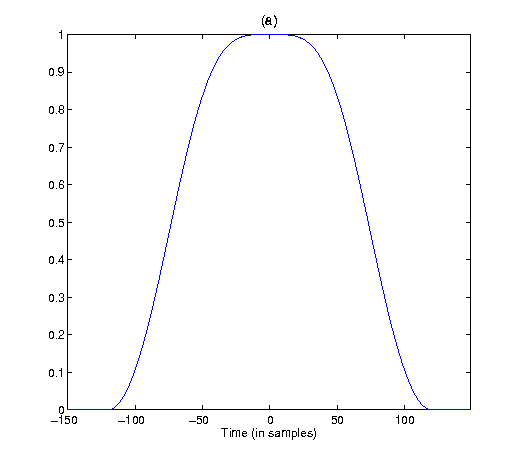
Analysis window in time domain
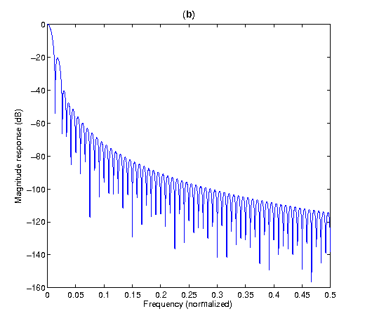
Analysis window in frequency domain
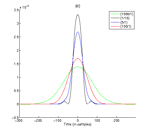
Results of optimization in the time domain
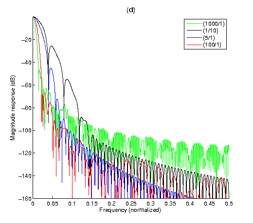
Results of optimization in the frequency domain
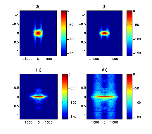
Results of optimization: ambiguity function
This code produces the following output:
Compute the canonical dual
  Reconstruction error of the canonical dual 2.4507e-16
Solve the optimization problem : 1/10
  Reconstruction error of optimization problem: 3.72352e-16
Solve the optimization problem : 3/1
  Reconstruction error of optimization problem: 5.4417e-16
Solve the optimization problem : 100/1
  Reconstruction error of optimization problem: 4.57452e-16
Solve the optimization problem : 1000/1
  Reconstruction error of optimization problem: 4.09409e-16

crit =

    0.2213    3.1216    3.6695    0.0215    1.7215    0.1220    1.4838    1.4359    1.5215    2.0074    0.5825
    0.7887    1.5032    0.6157    0.1385    0.8288    0.4349    1.5236    0.7754    2.0656    1.7002    1.2613
    0.5005    1.7009    1.0981    0.0473    0.9378    0.2760    1.3736    0.7669    1.7975    1.7394    0.9359
    0.2365    2.6391    3.3422    0.0082    1.4553    0.1304    1.4369    1.2506    1.5433    1.9631    0.5871
    0.1545    4.1818   10.9763    0.0114    2.3069    0.0852    1.7917    2.3180    1.5707    2.5117    0.4852


crit2 =

   24.5000    1.3958  292.4155   20.6072  129.5731    0.2213    3.1216
    8.1667    3.9375  310.9815   25.7860  153.8656    0.7887    1.5032
    9.8333    4.0208  252.9200   45.0251  161.5928    0.5005    1.7009
   18.5000    2.3125  233.7473   66.7578  103.8376    0.2365    2.6391
   28.1667    1.4792  240.0200   46.6063   71.2169    0.1545    4.1818


ans =

\begin{table}[thb]
\begin{center}\begin{tabular}{ |c|ccccccccccc|}
 \hline
 &  &  &  &  &  &  &  &  &  &  & \\\\
 \hline
 & :math:`   0.7887 ` & :math:`   1.5032 ` & :math:`   0.6157 ` & :math:`   0.1385 ` & :math:`   0.8288 ` & :math:`   0.4349 ` & :math:`   1.5236 ` & :math:`   0.7754 ` & :math:`   2.0656 ` & :math:`   1.7002 ` & :math:`   1.2613 ` \\\\
 & :math:`   0.5005 ` & :math:`   1.7009 ` & :math:`   1.0981 ` & :math:`   0.0473 ` & :math:`   0.9378 ` & :math:`   0.2760 ` & :math:`   1.3736 ` & :math:`   0.7669 ` & :math:`   1.7975 ` & :math:`   1.7394 ` & :math:`   0.9359 ` \\\\
 & :math:`   0.2365 ` & :math:`   2.6391 ` & :math:`   3.3422 ` & :math:`   0.0082 ` & :math:`   1.4553 ` & :math:`   0.1304 ` & :math:`   1.4369 ` & :math:`   1.2506 ` & :math:`   1.5433 ` & :math:`   1.9631 ` & :math:`   0.5871 ` \\\\
 & :math:`   0.1545 ` & :math:`   4.1818 ` & :math:`  10.9763 ` & :math:`   0.0114 ` & :math:`   2.3069 ` & :math:`   0.0852 ` & :math:`   1.7917 ` & :math:`   2.3180 ` & :math:`   1.5707 ` & :math:`   2.5117 ` & :math:`   0.4852 ` \\\\
 \hline
 \end{tabular}\end{center}
 \caption{ }
\end{table}


ans =

\begin{table}[thb]
\begin{center}\begin{tabular}{ |c|ccccccc|}
 \hline
 &  &  &  &  &  &  & \\\\
 \hline
 & :math:`   8.1667 ` & :math:`   3.9375 ` & :math:` 310.9815 ` & :math:`  25.7860 ` & :math:` 153.8656 ` & :math:`   0.7887 ` & :math:`   1.5032 ` \\\\
 & :math:`   9.8333 ` & :math:`   4.0208 ` & :math:` 252.9200 ` & :math:`  45.0251 ` & :math:` 161.5928 ` & :math:`   0.5005 ` & :math:`   1.7009 ` \\\\
 & :math:`  18.5000 ` & :math:`   2.3125 ` & :math:` 233.7473 ` & :math:`  66.7578 ` & :math:` 103.8376 ` & :math:`   0.2365 ` & :math:`   2.6391 ` \\\\
 & :math:`  28.1667 ` & :math:`   1.4792 ` & :math:` 240.0200 ` & :math:`  46.6063 ` & :math:`  71.2169 ` & :math:`   0.1545 ` & :math:`   4.1818 ` \\\\
 \hline
 \end{tabular}\end{center}
 \caption{ }
\end{table}