MODIFIED_PATH_COHERENCE - Illustrates how the relation between coherence and uncertainty

Description

This package contains the code to reproduce all the figures of the paper:

Global and Local Uncertainty Principles for Signals on Graphs

Authors: Nathanael Perraudin, Benjamin Ricaud, David I Shuman, Pierre Vandergheynst

ArXiv: http://arxiv.org/abs/1603.03030

Abstract of the paper

Uncertainty principles such as Heisenberg's provide limits on the time-frequency concentration of a signal, and constitute an important theoretical tool for designing and evaluating linear signal transforms. Generalizations of such principles to the graph setting can inform dictionary design for graph signals, lead to algorithms for reconstructing missing information from graph signals via sparse representations, and yield new graph analysis tools. While previous work has focused on generalizing notions of spreads of a graph signal in the vertex and graph spectral domains, our approach is to generalize the methods of Lieb in order to develop uncertainty principles that provide limits on the concentration of the analysis coefficients of any graph signal under a dictionary transform whose atoms are jointly localized in the vertex and graph spectral domains. One challenge we highlight is that due to the inhomogeneity of the underlying graph data domain, the local structure in a single small region of the graph can drastically affect the uncertainty bounds for signals concentrated in different regions of the graph, limiting the information provided by global uncertainty principles. Accordingly, we suggest a new way to incorporate a notion of locality, and develop local uncertainty principles that bound the concentration of the analysis coefficients of each atom of a localized graph spectral filter frame in terms of quantities that depend on the local structure of the graph around the center vertex of the given atom. Finally, we demonstrate how our proposed local uncertainty measures can improve the random sampling of graph signals.

Experiment 1

We start with a standard path graph of \(10\) nodes equally spaced (all edge weights are equal to one) and we move the first node out to the left; i.e., we reduce the weight between the first two nodes (see Figure 1). The weight is related to the distance by \(W_{12}=1/d(1,2)\) with \(d(1,2)\) being the distance between nodes 1 and 2. When the weight between nodes 1 and 2 decreases, the eigenvector associated with the largest eigenvalue of the Laplacian becomes more concentrated, which increases the coherence \(\mu_{G}\) (Figure 2).

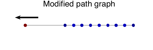
Example of a modified path graph with \(10\) nodes

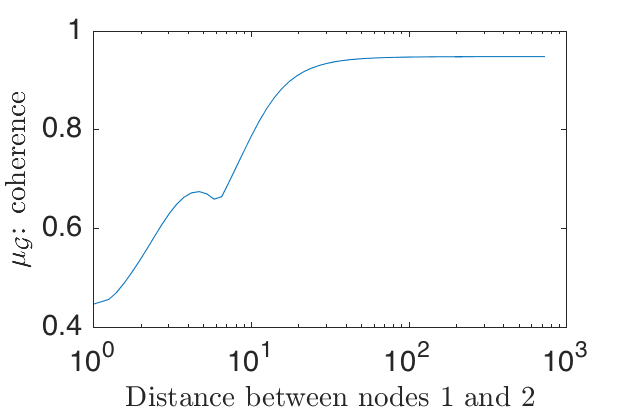
Graph coherence

Evolution of the coherence of the modified path graph with respect to the distance between nodes \(1\) and \(2\). As the degree of the comet's center vertex increases or the first node of the modified path is pulled away, the coherence \(\mu_{G}\) tends to the limit value \(\sqrt{\frac{N-1}{N}}\)

Experiment 2

Figure 3 shows the computation of the quantities involved in (1), with \(p=1\) and different graph's taken to be the modified path graphs of the modified path, with different distances between the first two vertices. We show the lefthand side of (1) for two different Kronecker deltas, one centered at vertex 1, and one centered at vertex 10. We have seen in global_illustration that as the distance between the first two vertices increases, the coherence increases, and therefore the lower bound on the right-hand side of (1) decreases. For \(\delta_1\), the uncertainty quantity on the left-hand side of (1) follows a similar pattern. The intuition behind this is that as the weight between the first two vertices decreases, a few of the eigenvectors start to have local jumps around the first vertex (see modified_path_eigenvectors ). As a result, we can sparsely represent \(\delta_1\) as a linear combination of those eigenvectors and \(||\widehat{\delta_1}||_1\) is reduced. However, since there are not any eigenvectors that are localized around the last vertex in the path graph, we cannot find a sparse linear combination of the graph Laplacian eigenvectors to represent \(\delta_{10}\). Therefore, its uncertainty quantity on the left-hand side of (1) does not follow the behavior of the lower bound.

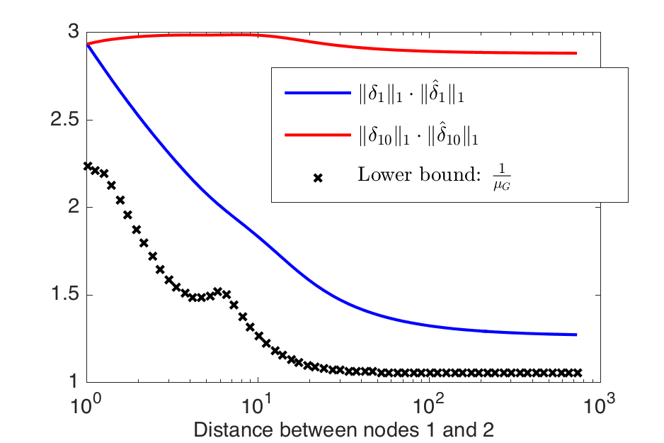
Evolution of bounds

Numerical illustration of the \(l^p\)-norm uncertainty principle on a sequence of modified path graphs with different mutual coherences between the canonical basis of deltas and the graph Laplacian eigenvectors. For each modified path graph, the weight \(W_{12}\) of the edge between the first two vertices is the reciprocal of the distance shown on the horizontal axis. The black crosses show the lower bound on the right-hand side of (1), with \(p=1\). The blue and red lines show the corresponding uncertainty quantity on the left-hand side of eqref{eq:rictorr}, for the graph signals \(\delta_1\) and \(\delta_{10}\), respectively.

Experiment 3

The Hausdorff-Young Theorem for graph signals is stated as:

Let \(\mu_{G}\) be the coherence between the graph Fourier and canonical bases of a graph \(G\). Let \(p,q>0\) be such that \(\frac{1}{p}+\frac{1}{q}=1\). For any signal \(f \in \mathbb{C}^N\) defined on \(G\) and \(1 \leq p \leq 2\), we have

and conversly:

Continuing with the modified path graphs, we illustrate the bounds of the Hausdorff-Young Hausdorff-Young Theorem. this example, we take the signal \(f\) to be \(\delta_1\), a Kronecker delta centered on the first node of the modified path graph. As a consequence, \(\|\delta_1\|_p=1\) for all \(p\), which makes it easier to compare the quantities involved in the inequalities. For this example, the bounds of Hausdorff-Young Theorem are fairly close to the actual values of \(\|\hat{\delta_1}\|_q\).

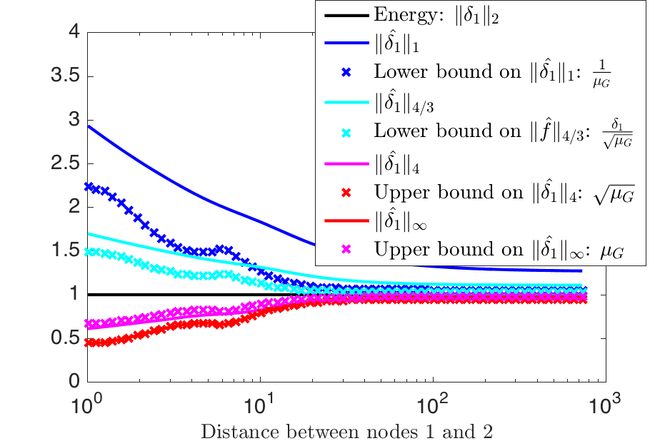
Illustration of the bounds of the Hausdorff-Young inequalities

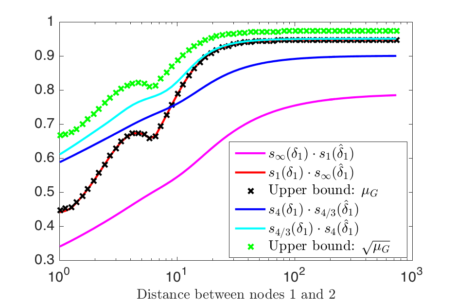
Illustration of the bounds of the Hausdorff-Young inequalities for graph signals on the modified path graphs with \(f=\delta_1\). The quantities in (2) and (3) for \(q=1,\frac{4}{3},4,\) and \(\infty\).

Illustration of the bounds of the Hausdorff-Young inequalities

The same quantities with respect of the sparsity level

References:

N. Perraudin, R. Benjamin, S. David I, and P. Vandergheynst. Global and local uncertainty principles for signals on graphs. arXiv preprint arXiv:1603.03030, 2016.