GSP_DEMO - Tutorial on the GSPBox
Description
In this demo, we are going to show the basic operations of the GSPBox. To lauch the toolbox, just go into the repository where the GSPBox was extracted and type:
gsp_start;
A banner will popup telling you that everything happens correctly. To speedup some processing, you might want to compile some mexfile. Refer to gsp_make for more informations. However, if the compilation is not working on your computer, keep quiet, everything should still work and most of the routine are implemented only in matlab.
Most likely, the first thing you would like to do is to create a graph. To do so, you only need the adjacendy or the weight matrix \(W\). Once you have it, you can construct a graph using:
G = gsp_graph(W);
This function will create a full structure ready to be used with the toolbox. To know a bit more about what is in this structure, you can refer to the help of the function gsp_graph_default_parameters.
The GSPBox contains also a list of graph generators. To see a full list of these graphs, type:
help graphs
This code produces the following output:
GSPBOX - Graphs

   Specific graphs
     gsp_swiss_roll              -  Create swiss roll graph
     gsp_david_sensor_network    -  Create the sensor newtwork from david
     gsp_ring                    -  Create the ring graph
     gsp_path                    -  Create the path graph
     gsp_airfoil                 -  Create the airfoil graph
     gsp_comet                   -  Create the comet graph
     gsp_erdos_renyi             -  Create a erdos renyi graph
     gsp_minnesota               -  Create Minnesota road graph
     gsp_low_stretch_tree        -  Create a low stretch tree graph
     gsp_sensor                  -  Create a random sensor graph
     gsp_random_regular          -  Create a random regular graph
     gsp_random_ring             -  Create a random ring graph
     gsp_full_connected          -  Create a fully connected graph
     gsp_nn_graph                -  Create a nearest neighbors graph
     gsp_rmse_mv_graph           -  Create a nearest neighbors graph with missing values
     gsp_sphere                  -  Create a spherical-shaped graph
     gsp_cube                    -  Create a cubical-shaped graph
     gsp_2dgrid                  -  Create a 2d-grid graph
     gsp_torus                   -  Create a torus graph
     gsp_logo                    -  Create a GSP logo graph
     gsp_community               -  Create a community graph
     gsp_bunny                   -  Create a bunny graph
     gsp_spiral                  -  Create a spiral graph
     gsp_stochastic_block_graph  -  Create a graph with the stochastic block model

   Hypergraphs
     gsp_nn_hypergraph           -  Create an hyper nearest neighbor graph
     gsp_hypergraph              -  Create an hypergraph

   Utils
     gsp_graph_default_parameters-  Initialise all parameters for a graph
     gsp_graph_default_plotting_parameters-  Initialise all plotting parameters for a graph
     gsp_graph                   -  Create a graph from a weight matrix
     gsp_update_weights          -  Update the weights of a graph
     gsp_update_coordinates      -  Update the coordinate of a graph
     gsp_components              -  Cuts non connected graph into several connected ones
     gsp_subgraph                -  Create a subgraph
     gsp_graph_product           -  Compute graph product between two graphs
     gsp_line_graph              -  Create the Line Graph (or edge-to-vertex dual graph) of a graph
     gsp_jtv_graph               -  Add time information to the graph structure


   For help, bug reports, suggestions etc. please send email to
   gspbox 'dash' support 'at' groupes 'dot' epfl 'dot' ch
For this demo, we will use the graph gsp_logo. You can load it using:
G = gsp_logo
This code produces the following output:
G =

  struct with fields:

             W: [1130×1130 double]
        coords: [1130×2 double]
          info: [1×1 struct]
      plotting: [1×1 struct]
        limits: [0 640 -400 0]
             A: [1130×1130 logical]
             N: 1130
          type: 'unknown'
      directed: 0
    hypergraph: 0
      lap_type: 'combinatorial'
             L: [1130×1130 double]
             d: [1130×1 double]
            Ne: 3131
Here observe the attribute of the structure G.
- G.W: Weight matrix
- G.A: Adacency matrix
- G.N: Number of nodes
- G.type: Type of graph
- G.directed: 1 if the graph is directed, 0 if not
- G.lap_type: Laplacian type
- G.d: Degree vector
- G.Ne: Number of edges
- G.coords: Coordinates of the vertices
- G.plotting: Plotting parameters
In the folder 'plotting', the GSPBox contains some plotting routine. For instance, we can plot a graph using:
gsp_plot_graph(G);

GSP graph
Wonderful! Isn't it? Now, let us start to analyse this graph. To compute graph Fourier transform or exact graph filtering, you need to precompute the Fourier basis of the graph. This operation could be relatively long since it involves a full diagonalization of the Laplacian. Don't worry, you do not need to perform this operation to filter signals on graph. The fourier basis is computed by:
G = gsp_compute_fourier_basis(G);
The function gsp_compute_fourier_basis add two new fields to the structure G:
- G.U: The eigenvectors of the Fourier basis
- G.e: The eigenvalues
The fourier eigenvectors does look like a sinusoide on the graph. Let's plot the second and the third ones. (The first one is constant!):
gsp_plot_signal(G,G.U(:,2));
title('Second eigenvector')
subplot(212)
gsp_plot_signal(G,G.U(:,3));
title('Third eigenvector')

Eigenvectors
Now, we are going to show a basic filtering operation. Filters are usually defined in the spectral domain. To define the following filter
just write in Matlab:
tau = 1;
h = @(x) 1./(1+tau*x);
Hint: You can define filterbank using cell array!
Let's display this filter:
gsp_plot_filter(G,h);
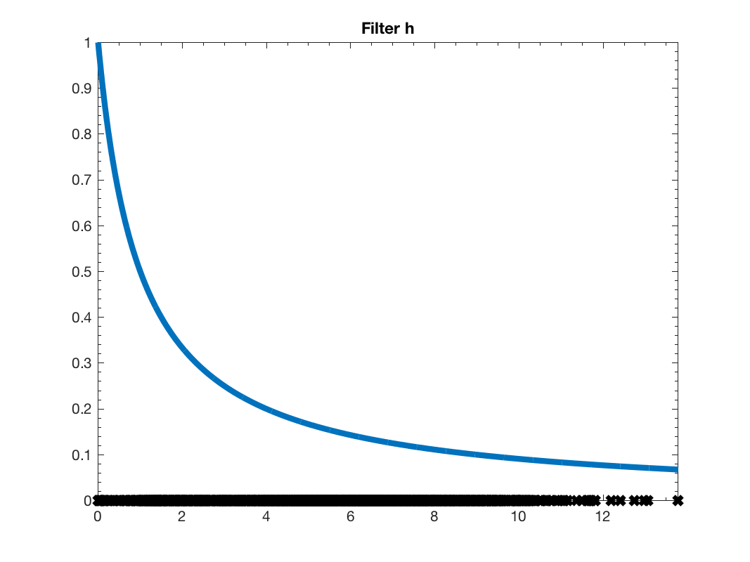
Low pass filter \(h\)
To apply the filter to a given signal, you only need to run a single function:
% Create a signal
f = zeros(G.N,1);
f(G.info.idx_g) = -1;
f(G.info.idx_s) = 1;
f(G.info.idx_p) = -0.5;
f = f + 0.3*randn(G.N,1);
% Remove the noise
f2 = gsp_filter(G,h,f);
gsp_filter is actually a shortcut to gsp_filter_analysis. gsp_filter_analysis performs the analysis operator associated to a filterbank. See the gsp_demo_wavelet for more information.
Finnaly, we display the result of this low pass filtering on the graph:
figure;
subplot(211)
gsp_plot_signal(G,f);
title('Signal with noise')
subplot(212)
gsp_plot_signal(G,f2);
title('Signal denoised');
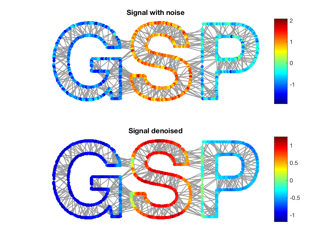
Result of filtering
Enjoy the GSPBOX !