GSP_DEMO_LEARN_GRAPH - Demonstration of learning a graph from data
Description
In this demo, we show how the graph learning can be used to learn a graph from smoothly changing signals. The theory behind the algorithm can be found in
[1] V. Kalofolias, How to learn a graph from smooth signals, AISTATS 2016.
[2] V. Kalofolias, N. Perraudin, Large Scale Graph Learning From Smooth Signals, ICLR 2019.
Suppose that we have some 2 dimensional smooth functions:
f1 = @(x,y) 20 * (-sin((2-x-y).^2)/2 + cos(y*3));
f2 = @(x,y) 30 * cos((x+y).^2);
f3 = @(x,y) 30 * ((x-.5).^2 + (y-.5).^3 + x - y);
f4 = @(x,y) 50 * sin(3*((x-.5).^2+(y-.5).^2));
and we have uniform samples as features, displayed below:
figure;
subplot(2,2,1); scatter(xc, yc, 700, X(:,1), '.');
title('1st smooth signal'); axis off; colorbar;
subplot(2,2,2); scatter(xc, yc, 700, X(:,2), '.');
title('2nd smooth signal'); axis off; colorbar;
subplot(2,2,3); scatter(xc, yc, 700, X(:,3), '.');
title('3rd smooth signal'); axis off; colorbar;
subplot(2,2,4); scatter(xc, yc, 700, X(:,4), '.');
title('4th smooth signal'); axis off; colorbar;
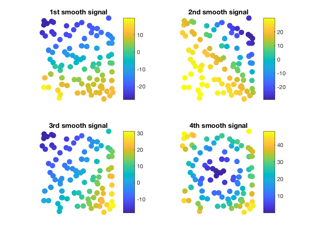
Different signals
We can compute the pairwise distances of the features and learn a graph using them:
Z1 = gsp_distanz(X(:, 1)').^2;
W1 = gsp_learn_graph_log_degrees(Z1, 1.5, 1, params);
The second parameter penalizes the formation of un-connected nodes, and the third penalizes the formation of too strong weights. We then clean any tiny edges (due to numerical error), to obtain a sparse weighted adjacency matrix. We feed this to gsp_graph to create a graph with the given coordinates and weights:
W1(W1<1e-5) = 0;
G1 = gsp_graph(W1, [xc, yc]);
We can also update the weights of an already existing graph using gsp_update_weights. If we learn the graphs of all four above functions, we get quite different results:
figure;
subplot(2,2,1); gsp_plot_edges(G1, params_plot);
title('graph learned from 1st smooth signal');
subplot(2,2,2); gsp_plot_edges(G2, params_plot);
title('graph learned from 2nd smooth signal');
subplot(2,2,3); gsp_plot_edges(G3, params_plot);
title('graph learned from 3rd smooth signal');
subplot(2,2,4); gsp_plot_edges(G4, params_plot);
title('graph learned from 4th smooth signal');
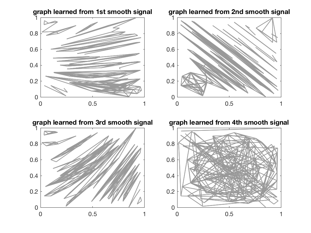
Different graphs learned
Note that the edges follow the level curves of the above functions.
If we use all four above smooth functions as features to learn the graph:
Z = gsp_distanz(X').^2;
W = gsp_learn_graph_log_degrees(Z/500, 2, 1, params);
we get a result that has more local edges:
params_plot.show_edges = 1;
G.plotting.vertex_size = 5;
figure; gsp_plot_graph(G, params_plot);
title('Graph with edges learned from above 4 signals');
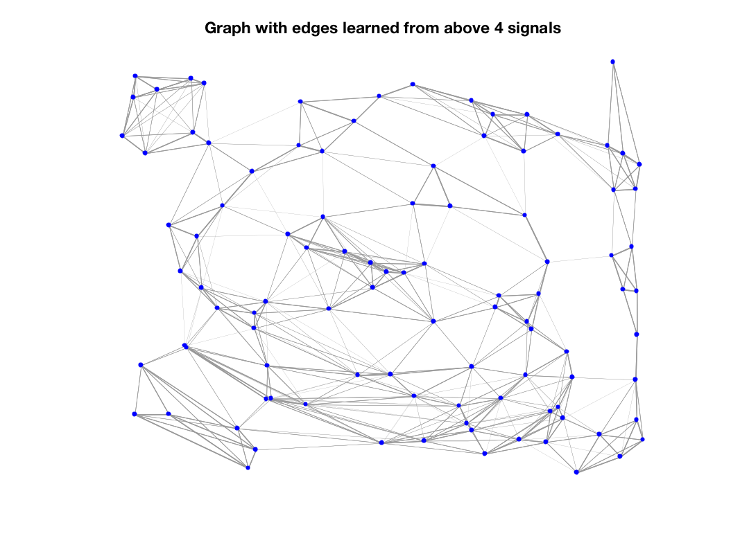
Graph with edges learned from above 4 signals
This is close to the graph that we would learn using the acutal coordinates as features. So why does it work so well? We can see that the pattern of the pairwise distances using these features is similar to the one of the pairwise geometric distances between nodes:
figure;
subplot(1, 2, 1);
imagesc(gsp_distanz(X'));
title('Geometric pairwise distances between nodes');
subplot(1, 2, 2);
imagesc(gsp_distanz([xc, yc]'));
title('Pairwise distances computed from features');
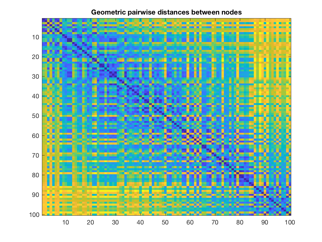
Geometric pairwise distances between nodes
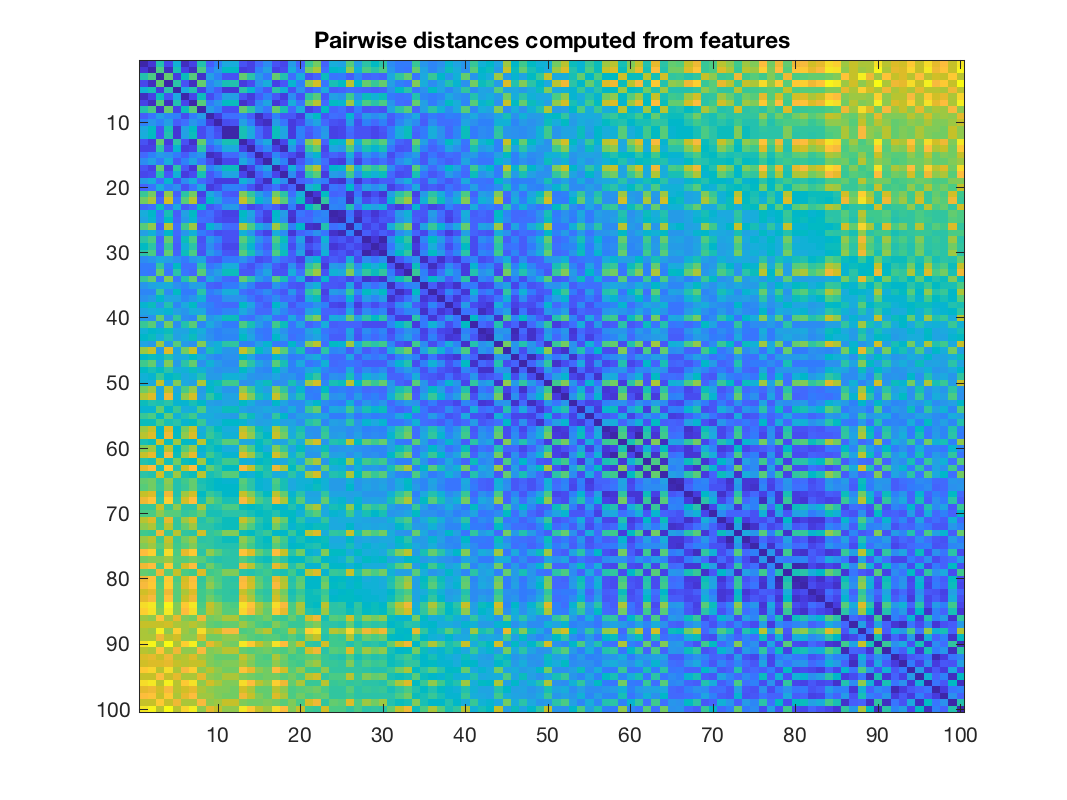
Pairwise distances computed from features
The functions available for learning a graph are gsp_learn_graph_log_degrees and gsp_learn_graph_l2_degrees.
This code produces the following output:
# iters: 3226. Rel primal: 3.0817e-06 Rel dual: 9.9911e-06  OBJ 1.171e+01
Time needed is 0.565373 seconds
# iters: 21427. Rel primal: 8.0025e-06 Rel dual: 9.9949e-06  OBJ -2.239e+02
Time needed is 3.051031 seconds
# iters: 1818. Rel primal: 5.9225e-06 Rel dual: 9.9869e-06  OBJ -9.442e+02
Time needed is 0.265353 seconds
# iters: 2173. Rel primal: 7.7403e-06 Rel dual: 9.9829e-06  OBJ -4.585e+01
Time needed is 0.310343 seconds
# iters:  754. Rel primal: 9.5232e-06 Rel dual: 9.9831e-06  OBJ -1.749e+02
Time needed is 0.108606 seconds
Graph of signal 1: 213  edges
Graph of signal 2: 263  edges
Graph of signal 3: 232  edges
Graph of signal 4: 197  edges
Graph of all signals: 439  edges
References:
V. Kalofolias. How to learn a graph from smooth signals. Technical report, AISTATS 2016: proceedings at Journal of Machine Learning Research (JMLR)., 2016.
V. Kalofolias and N. Perraudin. Large scale graph learning from smooth signals. International Conference on Learning Representations, 2019. [ http ]