This is where navigation should be.
GSP_DESIGN_MEXICAN_HAT - Design the mexican hat filterbank
Usage
g =  gsp_design_mexican_hat(G, Nf, param);
gsp_design_mexican_hat(G ,Nf);
gsp_design_mexican_hat(G);
Input parameters
| G | Graph or upper bound on the Laplacian spectrum |
| Nf | Number of filters to cover the interval [0,lmax] (default 6) |
| param | Structure of optional parameters |
Output parameters
| g | A cell array of filters |
Description
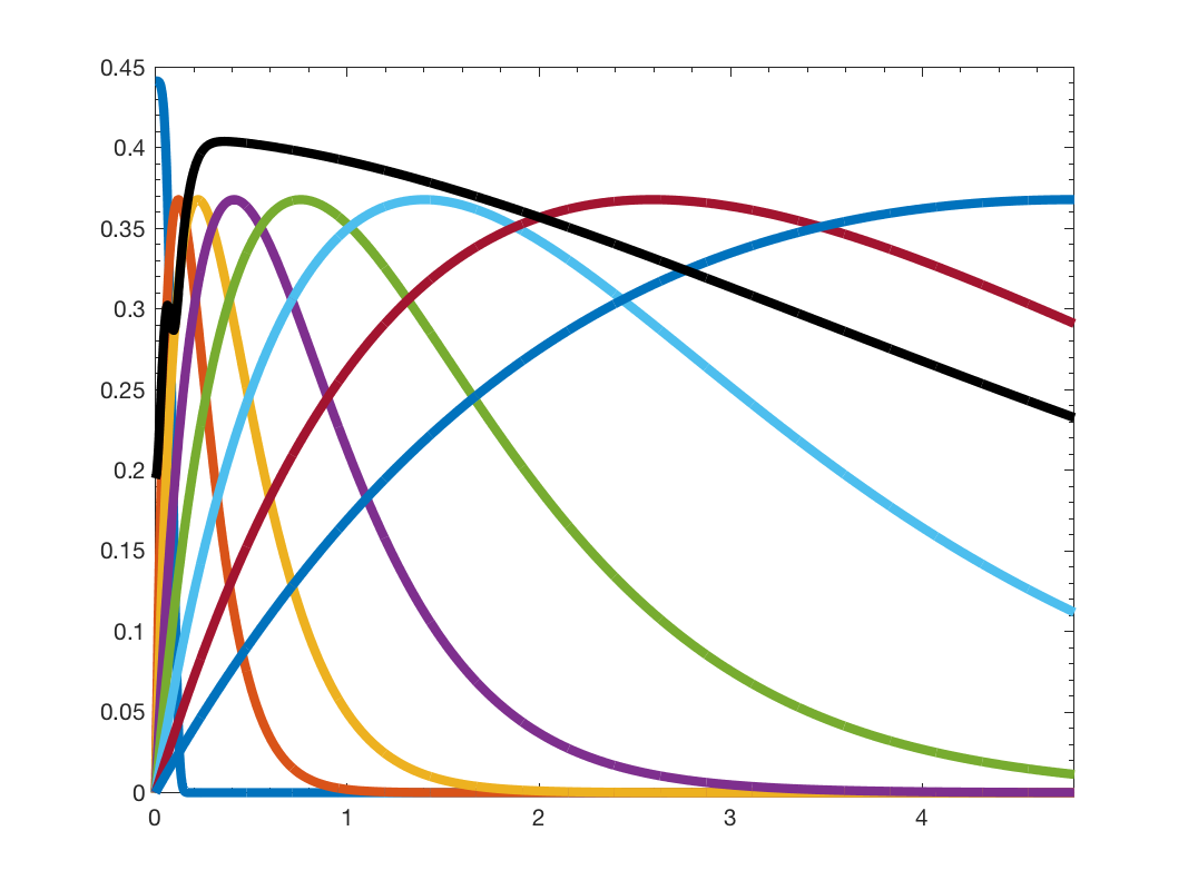
This function return a array of filters designed to be mexican hat wavelet. The mexican hat wavelet is the second oder derivative of a Gaussian. Since we express the filter in the Fourier domain, we find:
In our convention the eigenvalues of Laplacian are equivalent to the square of vertex frequencies: \(f = \lambda^2\).
The low pass filter is given by
param is an optional structure containing the following fields
- param.t: vector of scale to be used (default: log scale)
- param.lpfactor: lmin*=*lmax/lpfactor will be used to determine scales, then scaling function kernel will be created to fill the lowpass gap. (default 20)
- param.verbose: verbosity level. 0 no log - 1 display warnings. (default 1)
- param.normalize: normalize the wavelet by the factor \(\sqrt{t}\) (default 0.)
This function will compute the maximum eigenvalue of the laplacian. To be more efficient, you can precompute it using:
G = gsp_estimate_lmax(G);
Example:
Nf = 8;
G = gsp_sensor(100);
G = gsp_estimate_lmax(G);
g = gsp_design_mexican_hat(G, Nf);
gsp_plot_filter(G,g);

This function is inspired by the sgwt_toolbox.